Calculate an OLS regression using matrices in Python using Numpy

The following code will attempt to replicate the results of the numpy.linalg.lstsq() function in Numpy. For this exercise, we will be using a cross sectional data set provided by me in .csv format called “cdd.ny.csv”, that has monthly cooling degree data for New York state. The data is available here (File –> Download).

The OLS regression equation:

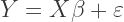
where a white noise error term. For this example the population-weighted Cooling Degree Days (CDD) (CDD.pop.weighted), and CDD measured at La Guardia airport (CDD.LGA). Note: this is a meaningless regression used solely for illustrative purposes.

Recall that the following matrix equation is used to calculate the vector of estimated coefficients of an OLS regression:

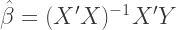
where the matrix of regressor data (the first column is all 1’s for the intercept), and the vector of the dependent variable data.

Matrix operators in Numpy

• matrix() coerces an object into the matrix class.
• .T  transposes a matrix.
• * or dot(X,Y) is the operator for matrix multiplication (when matrices are 2-dimensional; see here).
• .I takes the inverse of a matrix. Note: the matrix must be invertible.

Back to OLS

The following code calculates the 2 x 1 matrix of coefficients, :

## load in required modules:
import numpy as np
import csv

## read data into a Numpy array
df1 = csv.reader(open('/your/file/path/cdd.ny.csv', 'rb'),delimiter=',')
b1 = np.array(list(df1))[1:,3:5].astype('float')

nrow = b1.shape[0]

intercept = np.ones( (nrow,1) )
b2 = b1[:,0].reshape(-1, 1)

X = np.concatenate((intercept, b2), axis=1)
Y = b1[:,1].T

## X and Y arrays must have the same number of columns for the matrix multiplication to work:
print(X.shape)
print(Y.shape)

## Use the equation above (X'X)^(-1)X'Y to calculate OLS coefficient estimates:
bh = np.dot(np.linalg.inv(np.dot(X.T,X)),np.dot(X.T,Y))
print bh

## check your work with Numpy's built in OLS function:
z,resid,rank,sigma = np.linalg.lstsq(X,Y)
print(z)

Calculating Standard Errors

To calculate the standard errors, you must first calculate the variance-covariance (VCV) matrix, as follows:

The VCV matrix will be a square k x k matrix. Standard errors for the estimated coefficients are found by taking the square root of the diagonal elements of the VCV matrix.

## Calculate vector of residuals
res = as.matrix(women$weight-bh[1]-bh[2]*women$height)
res = Y-(bh[0]+X[:,1]*bh[1])
## Define n and k parameters
n = nrow
k = X.shape[1]

## Calculate Variance-Covariance Matrix
VCV = np.true_divide(1,n-k)*np.dot(np.dot(res.T,res),np.linalg.inv(np.dot(X.T,X)))

## Standard errors of the estimated coefficients
stderr = np.sqrt(np.diagonal(VCV))

Now you can check the results above using the lm() function in R:

df1 = read.csv('/your/file/path/cdd.ny.csv',header=T)
coef(lm(CDD.pop.weighted ~ CDD.LGA,data=df1))

## (Intercept) CDD.LGA
## -7.6210191 0.5937734

summary(lm(CDD.pop.weighted ~ CDD.LGA,data=df1))